

PyAT Primer#
Introduction#
The Accelerator Toolbox (AT) is a toolbox of functions in Matlab for charged particle beam simulation. It was created by Andrei Terebilo in the late 1990’s. The original papers[1][2] still serve as a good introduction to AT. The AT described in those papers is AT1.3, the latest version produced by Terebilo. The next version of AT is considered AT2.0[3]. Here we provide examples showing some of the changes from AT1.3, but also serving as an introduction for someone just starting AT.
AT Coordinate system#
The AT coordinate system is based on a design trajectory along which the magnetic elements are aligned, and a reference particle:
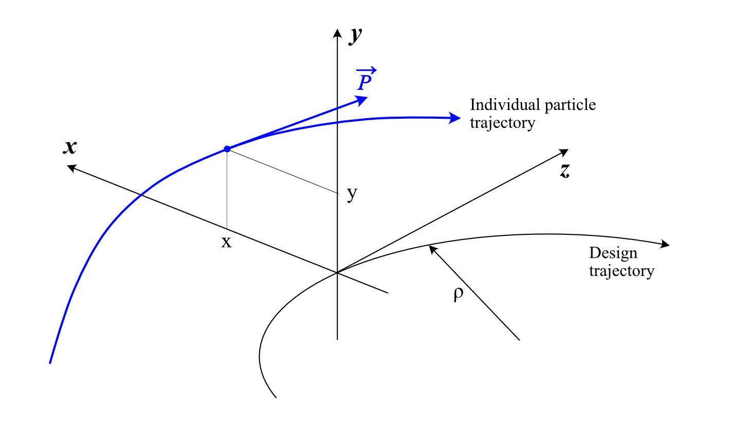
By convention, the reference particle travels along the design trajectory at constant nominal energy and defines the phase origin of the RF voltage.
The 6-d coordinate vector \(\vec Z\) is:
\(p_0\) is the reference momentum.
AT works with relative path lengths: the 6th coordinate \(\beta c\tau\) represents the path lengthening with respect to the reference particle. \(\tau\) is the delay with respect to the reference particle: the particle is late for \(\tau > 0\).
Creation of Elements and Lattices#
import at
import at.plot
import numpy as np
import matplotlib as mpl
import matplotlib.pyplot as plt
from math import pi
A lattice in AT is a object of the Lattice class containing the lattice elements. These elements may be created using element creation functions. These functions output objects inheriting from the Element base class. For example, a quadrupole may be created with the function Quadrupole.
QF = at.Quadrupole("QF", 0.5, 1.2)
print(QF)
Quadrupole:
       FamName: QF
        Length: 0.5
    PassMethod: StrMPoleSymplectic4Pass
      MaxOrder: 1
   NumIntSteps: 10
      PolynomA: [0. 0.]
      PolynomB: [0.  1.2]
             K: 1.2
We note that the family name of this quadrupole is ’QF’ and the pass
method is QuadMPoleFringePass. The fields following are parameters
necessary to be able to pass an electron through this quadrupole (i.e.,
the set of arguments required by the pass method). We now create some
other elements needed in a FODO lattice:
Dr = at.Drift("Dr", 0.5)
HalfDr = at.Drift("Dr2", 0.25)
QD = at.Quadrupole("QD", 0.5, -1.2)
Bend = at.Dipole("Bend", 1, 2 * pi / 40)
In addition to Quadrupole that we already saw, we have created a
drift (region with no magnetic field), using Drift. Besides the
family name, the only other needed field is the length. Since we split
the cell in the center of the drift, we have also created a half drift
element. The drifts are 0.5 meters long and the half drift is 0.25
meters long. We have defined a sector dipole, or bend magnet using
Dipole. The family name is ’Bend’. The second field is the length
of the magnet and we have given it a length of 1 meter. Next is the
bending angle. We have defined just an arc of a FODO lattice here, so we
don’t have to bend by all of \(2\pi\) here. We choose to have 20 total
such arcs, for a realistic field strength, and thus we define the
bending angle to be \(2\pi/40\) since there are two bends per cell.
A cell of a FODO lattice may now be constructed as follows
FODOcell = at.Lattice(
    [HalfDr, Bend, Dr, QF, Dr, Bend, Dr, QD, HalfDr],
    name="Simple FODO cell",
    energy=1e9,
)
print(FODOcell)
Lattice(<9 elements>, name='Simple FODO cell', energy=1000000000.0, particle=Particle('relativistic'), periodicity=1, beam_current=0.0, nbunch=0)
Attention
When repeating the same element in a Lattice, like Dr or Bend in FODOcell, all occurences refer to the same element, so any modification of the first drift will also affect the second one.
As mentioned, this cell is only 1/20 of a FODO lattice. The entire lattice may be created by repeating this cell 20 times as follows
FODO = FODOcell * 20
print(FODO)
Lattice(<180 elements>, name='Simple FODO cell', energy=1000000000.0, particle=Particle('relativistic'), periodicity=1, beam_current=0.0, nbunch=0)
We have now created a valid AT lattice, using drifts, dipoles, and quadrupoles.
Important
Contrary to the standard python list, the *operator on Lattices makes deep copies of
elements to populate to result, so that the final Lattice has independent elements
Common AT element classes are defined in the module at.lattice.elements.
We will later add some sextupoles to this lattice, and also an RF cavity, but one could already track particles through this lattice, as is.
Lattice Querying and Manipulation#
There are many parameters in a storage ring lattice. We need tools to view these parameters and to change them.
Selecting elements#
We have seen how to concatenate elements to form a lattice. To extract elements, two indexing methods may be used, similar to indexing in numpy arrays:
Integer array indexing: elements are identified by the array of their indices. For instance, the elements at locations 3 and 7 of
FODOcellmay be selected with:
list(FODOcell[3, 7])
[Quadrupole('QF', 0.5, 1.2), Quadrupole('QD', 0.5, -1.2)]
Boolean array indexing; elements are identified by a Boolean array, as long as the Lattice, where selected elements are identified by a True value. The same elements as in the previous example may be selected with:
mask = np.zeros(len(FODOcell), dtype=bool)
mask[3] = True
mask[7] = True
list(FODOcell[mask])
[Quadrupole('QF', 0.5, 1.2), Quadrupole('QD', 0.5, -1.2)]
Indexing can also be performed with string patterns using shell-style wildcards
(see fnmatch). This indexes elements based ob the FamName attribute:
list(FODOcell["Q[FD]"])
[Quadrupole('QF', 0.5, 1.2), Quadrupole('QD', 0.5, -1.2)]
We can also index elements according to their type:
list(FODOcell[at.Drift])
[Drift('Dr2', 0.25),
 Drift('Dr', 0.5),
 Drift('Dr', 0.5),
 Drift('Dr', 0.5),
 Drift('Dr2', 0.25)]
Many AT function have an input argument, usually named refpts using such indexing methods to select the “points of interest” in the function output. Please note that:
The corresponding locations in the ring are the entrances of the selected ring elements,
as a special case, a value of “len(ring)” (normally out-of-range element) is used to indicate the exit of the last element (think of it as the entrance of the 2nd turn).
Special constants are available to refer to commonly used locations:
Allrefers to all the available locations (equivalent torange(len(ring)+1)),Endrefers to the exit of the last element (equivalent tolen(ring)),Nonemeans no selected element (equivalent to[].
Integer or boolean indices can be generated with the Lattice.get_bool_index() method, which returns a boolean index of selected elements and Lattice.get_uint32_index() which returns an integer index.
refquad = FODOcell.get_bool_index(at.Quadrupole)  # All quadrupoles
print(refquad)
refqd = FODOcell.get_bool_index("QD")  # FamName attribute == QD
print(refqd)
[False False False  True False False False  True False False]
[False False False False False False False  True False False]
Boolean indices can be combined for complex selections:
refbend = FODOcell.get_bool_index(at.Dipole)  # All dipoles
print(list(FODOcell[ refquad | refbend]))  # All dipoles and quadrupoles
[Dipole('Bend', 1.0, 0.15707963267948966, 0.0), Quadrupole('QF', 0.5, 1.2), Dipole('Bend', 1.0, 0.15707963267948966, 0.0), Quadrupole('QD', 0.5, -1.2)]
Iterating over selected elements#
The Lattice.select() method of the lattice object returns an iterator over the selected elements:
for elem in FODOcell.select(at.Quadrupole):
    print(elem)
Quadrupole:
       FamName: QF
        Length: 0.5
    PassMethod: StrMPoleSymplectic4Pass
      MaxOrder: 1
   NumIntSteps: 10
      PolynomA: [0. 0.]
      PolynomB: [0.  1.2]
             K: 1.2
Quadrupole:
       FamName: QD
        Length: 0.5
    PassMethod: StrMPoleSymplectic4Pass
      MaxOrder: 1
   NumIntSteps: 10
      PolynomA: [0. 0.]
      PolynomB: [ 0.  -1.2]
             K: -1.2
Extracting attribute values#
Following the previous example, we can get the quadrupole strengths (PolynomB[1]) with:
np.array([elem.PolynomB[1] for elem in FODOcell.select(refquad)])
array([ 1.2, -1.2])
The same result is provided by the get_value_refpts() convenience function:
at.get_value_refpts(FODOcell, "Q[FD]", "PolynomB", index=1)
array([ 1.2, -1.2])
Setting attribute values#
Similarly, using a the Lattice iterator, we can write:
new_strengths = [1.1, -1.3]
for elem, strength in zip(FODOcell.select(refquad), new_strengths):
    elem.PolynomB[1] = strength
# Check the result:
np.array([elem.PolynomB[1] for elem in FODOcell.select(refquad)])
array([ 1.1, -1.3])
Or with the set_value_refpts() function:
initial_strengths = [1.2, -1.2]
at.set_value_refpts(FODOcell, refquad, "PolynomB", initial_strengths, index=1)
# Check the result:
at.get_value_refpts(FODOcell, refquad, "PolynomB", index=1)
array([ 1.2, -1.2])
Tracking#
Once a lattice is defined, electrons may be tracked through it.
The Lattice.track() method does that. An example of its
use is as follows:
nturns = 200
Z01 = np.array([0.001, 0, 0, 0, 0, 0])
Z02 = np.array([0.002, 0, 0, 0, 0, 0])
Z03 = np.array([0.003, 0, 0, 0, 0, 0])
Z1, *_ = FODO.track(Z01, nturns)
Z2, *_ = FODO.track(Z02, nturns)
Z3, *_ = FODO.track(Z03, nturns)
fig, ax = plt.subplots()
ax.plot(Z1[0, 0, 0, :], Z1[1, 0, 0, :], ".")
ax.plot(Z2[0, 0, 0, :], Z2[1, 0, 0, :], ".")
ax.plot(Z3[0, 0, 0, :], Z3[1, 0, 0, :], ".")
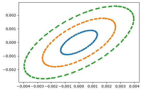
In this example, we started with one initial condition, and all subsequent turns are returned by Lattice.track(). We may also start with multiple initial conditions:
Z0 = np.asfortranarray(np.vstack((Z01, Z02, Z03)).T)
print("Z0.shape:", Z0.shape)
Z, *_ = FODO.track(Z0, nturns)
print(" Z.shape:", Z.shape)
Z0.shape: (6, 3)
 Z.shape: (6, 3, 1, 200)
Now the same plot can be obtained with:
fig, ax = plt.subplots()
ax.plot(Z[0, 0, 0, :], Z[1, 0, 0, :], ".")
ax.plot(Z[0, 1, 0, :], Z[1, 1, 0, :], ".")
ax.plot(Z[0, 2, 0, :], Z[1, 2, 0, :], ".")
Computation of beam parameters#
Now that particles can be tracked through the lattice, we can use the
tracking to understand different properties of the lattice. First, we
would like to understand the linear properties such as Twiss parameters,
tunes, chromaticities, etc. These can all be calculated with the
function get_optics().
[_, beamdata, _] = at.get_optics(FODO, get_chrom=True)
The first argument is the FODO lattice we have created. The second argument says we want to compute the optional chromaticity.
print(beamdata.tune)
print(beamdata.chromaticity)
[0.21993568 0.91777806]
[-6.3404156  -6.19856968]
which tells us the tunes are \(\nu_x = 0.2199\) and \(\nu_y = 0.9178\) and the chromaticities are \(\xi_x = -6.34\), \(\xi_y = -6.20\).
How did AT calculate these quantities? Without digging into the details of get_optics(), you could still figure it out, just based on the ability to track with the Lattice.track() function. In fact, AT computes the one-turn transfer matrix by tracking several initial conditions and interpolating. The one turn transfer matrix (here we focus on 4x4) is computed with the function find_m44() contained within get_optics(). Calling this on the FODO lattice, we find
m44, _ = at.find_m44(FODO, 0)
print(m44)
[[-0.6518562   1.90977797  0.          0.        ]
 [-0.87430341  1.02741279  0.          0.        ]
 [ 0.          0.         -0.1807342  -3.24829821]
 [ 0.          0.          0.41466639  1.91972581]]
The 0 as the second argument tells us to compute with \(\delta=0\). We
note that the ring is uncoupled, and computing the eigenvalues of
submatrices, we derive the tunes reported in get_optics() above.
Computing the tunes with varying \(\delta\) allows the computation of the chromaticity.
Now, suppose we would like to change the tunes in our FODO lattice. We know that we should change the quadrupole strengths, but we may not know exactly what values to use.
Here we reach the question of tuning. How do we set the parameters for
these quadrupoles in order to correct the tunes? In principle we have
the tools that we need. We can set the values of the quadrupoles using
the function set_value_refpts() and then recompute the chromaticity with
get_optics(). But we still don’t know what values to actually give the
quadrupoles. One could compute the value, or instead use an optimization
routine to vary the values until the correct output tunes are achieved.
This is the approach followed with the function fit_tune().
This allows you to vary quadrupole strengths until the desired tune values are reached. It is used as follows:
First, we need to select two variable quadrupoles families:
refqf = at.get_cells(FODO, at.checkname("QF"))  # Select all QFs
refqd = at.get_cells(FODO, at.checkname("QD"))  # Select all QDs
Then we can call the fitting function to set the tunes to \(\nu_x = 0.15\) and \(\nu_y = 0.75\) using the quadrupoles QF and QD.
at.fit_tune(FODO, refqf, refqd, [0.15, 0.75])
Fitting Tune...
Initial value [0.21993568 0.91777806]
iter# 0 Res. 1.8554910834426122e-06
iter# 1 Res. 7.129086923898827e-10
iter# 2 Res. 2.6680040922450136e-13
Final value [0.1500004  0.75000033]
Let’s check the result:
[_, beamdata, _] = at.get_optics(FODO)
beamdata.tune
array([0.1500004 , 0.75000033])
Giving satisfactory results for the tunes.
Now, in case you have some experience with storage ring dynamics, you will know that these negative chromaticity values will lead to instability and thus our FODO lattice, as is, is not acceptable. To fix this problem, we add sextupoles to our lattice. We define a focusing and defocussing sextupoles (0.1 meter long) as follows:
SF = at.Sextupole("SF", 0.1, 0)
SD = at.Sextupole("SD", 0.1, 0)
drs = at.Drift("DRS", 0.2)
Now we want to add these to the lattice at locations where they will be effective. We will put them in the middle of the 0.5 meter drift sections: SF before the QF and SD before the QD. Let’s locate the drifts:
FODOcell.get_uint32_index("Dr")
array([2, 4, 6], dtype=uint32)
We will insert SF in the middle of element 2 and SD in the middle of element 6. Since the Lattice object is derived from the python list, we can use all the list methods to do this. For instance:
FODOcellSext = FODOcell.copy()
FODOcellSext[6:7] = [drs, SD, drs]
FODOcellSext[2:3] = [drs, SF, drs]
FODOSext = FODOcellSext * 20
print(FODOSext)
Lattice(<260 elements>, name='Simple FODO cell', energy=1000000000.0, particle=Particle('relativistic'), periodicity=1, beam_current=0.0, nbunch=0)
[_, beamdata, _] = at.get_optics(FODOSext, get_chrom=True)
print(beamdata.tune)
print(beamdata.chromaticity)
[0.21993568 0.91777806]
[-6.34041563 -6.19856968]
The tunes of FODOSext are identical to the ones of FODO. Now we need to tune the sextupoles. For this, we will use the function fit_chrom(). This function works analogously to fit_tune() except the sextupoles are varied instead of the quadrupoles. Let’s locate the first sextupoles:
refsext = FODOSext.get_bool_index(at.Sextupole)  # Select all sextpoles
refsf, refsd = np.flatnonzero(refsext)[:2]  # Take the 1st ones
at.fit_chrom(FODOSext, refsf, refsd, [0.5, 0.5])
Fitting Chromaticity...
Initial value
[-6.34041563 -6.19856968]
iter# 0 Res. 0.0001897928049993579
iter# 1 Res. 5.750045391368994e-10
iter# 2 Res. 1.5649357129107472e-15
Final value [0.49999996 0.5       ]
After changing the tunes and fixing the chromaticities, we find:
[_, beamdata, _] = at.get_optics(FODOSext, get_chrom=True)
print(beamdata.tune)
print(beamdata.chromaticity)
[0.21993568 0.91777806]
[0.49999996 0.5       ]
You may have noticed that we ignored two outputs of fit_tune(). They contains linear optics parameters that vary around the ring. These are the Twiss parameters, dispersions, phase advance, and coupling parameters. elemdata0 is their values at the entrance of the ring, elemdata is the values at the selected points of interest. To compute them at all lattice elements, we call:
[elemdata0, beamdata, elemdata] = at.get_optics(
    FODOcellSext, range(len(FODOcellSext) + 1)
)
Examining elemdata, we find:
print("elemdata.shape:", elemdata.shape)
print("elemdata.fields:")
for fld in elemdata.dtype.fields.keys():
    print(fld)
elemdata.shape: (14,)
elemdata.fields:
alpha
beta
mu
R
A
dispersion
closed_orbit
M
s_pos
’s_pos’ is the set of \(s\) positions,
’closed_orbit’ is the \(x,p_x,y,p_y\) coordinate vector of the closed orbit,
’dispersion’ is the \(\eta_x,\eta'_x,\eta_y,\eta'_y\) coordinate vector of the dispersion,
’M’ is the local \(4\times 4\) transfer matrix,
’beta’ gives the horizontal and vertical \(\beta\) functions,
’alpha’ gives the Twiss parameters \(\alpha_{x,y}\),
’mu’ gives the phase advances (times \(2\pi\)).
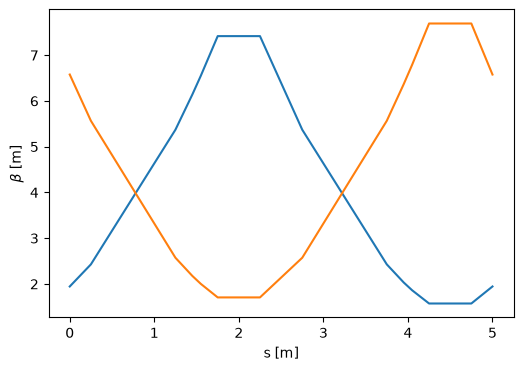
Let us use these results to plot the beta functions around the ring.
plt.plot(elemdata.s_pos, elemdata.beta)
plt.xlabel("s [m]")
plt.ylabel(r"$\beta$ [m]");
We may also plot the lattice parameters using a dedicated plot function with the command:
FODOcellSext.plot_beta();
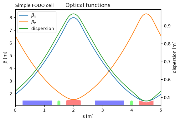
Note that the magnets are displayed below the function, giving a convenient visualization. Also note that the lattice functions are smoother than those we saw before. They have been computed at more positions, by slicing the magnets in the plot_beta() function.
Beam sizes#
The parameters computed thus far use only the tracking through the
lattice, with no radiation effects. In reality, for electrons, we know
that there are radiation effects which cause a damping and diffusion and
determine equilibrium emittances and beam sizes. This is computed in AT
by the ohmi_envelope() function using the Ohmi envelope formalism.
In order to use ohmi_envelope(), we first need to make sure the beam is stable
longitudinally as well, requiring us to add an RF cavity to our FODO
lattice. Let’s add an inactive cavity with the command
RFC = at.RFCavity("RFC", 0.0, 0.0, 0.0, 1, 1.0e9, PassMethod="IdentityPass")
FODOSext.insert(0, RFC)
FODOSext.harmonic_number = 100
Now, we need to set the values of the RF cavity. This can be done with
the function set_cavity() as follows:
FODOSext.set_cavity(Voltage=0.5e6, Frequency=at.Frf.NOMINAL)
print(RFC)
RFCavity:
       FamName: RFC
        Length: 0.0
    PassMethod: IdentityPass
        Energy: 1000000000.0
     Frequency: 2997924.5799999973
    HarmNumber: 1
       TimeLag: 0.0
       Voltage: 500000.0
which says that the each of the 20 RF cavities has a voltage of 25 kV.
radiation_parameters() gives a summary of the lattice properties, using the classical radiation integrals:
print(at.radiation_parameters(FODOSext))
              Frac. tunes: [0.21993568 0.91777806 0.01826495]
                    Tunes: [5.21993568 4.91777806]
           Chromaticities: [0.49999996 0.5       ]
 Momentum compact. factor: 4.193890e-02
              Slip factor: -4.193864e-02
                   Energy: 1.000000e+09 eV
       Energy loss / turn: 1.389569e+04 eV
 Radiation integrals - I1: 4.1938903743693405 m
                       I2: 0.9869604401089351 m^-1
                       I3: 0.15503138340149902 m^-2
                       I4: 0.10348009724140478 m^-1
                       I5: 0.020256990008554306 m^-1
          Mode emittances: [3.36477905e-08            nan 4.00215446e-06]
Damping partition numbers: [0.89515274 1.         2.10484726]
            Damping times: [0.05363298 0.04800971 0.02280912] s
            Energy spread: 0.000330932
             Bunch length: 0.0120936 m
         Cavities voltage: 500000.0 V
        Synchrotron phase: 3.1138 rd
    Synchrotron frequency: 54756.9 Hz
We may now turn radiation ON and call the function ohmi_envelope() as follows
FODOSext.enable_6d()
_, beamdata, _ = at.ohmi_envelope(FODOSext)
print("beamdata.fields:")
for fld in beamdata.dtype.fields.keys():
    print(fld)
beamdata.fields:
tunes
damping_rates
mode_matrices
mode_emittances
’tunes’ gives the 3 tunes of the 6D motion;
’damping_rates’,
’mode_matrices’ are the sigma matrices of the 3 independent motions
’mode_emittances’ are the 3 modal emittances.
An easy way to summarize these results is provided by the envelope_parameters() function:
print(at.envelope_parameters(FODOSext))
  Frac. tunes (6D motion): [0.21997027 0.91788601 0.0018265 ]
                   Energy: 1.000000e+09 eV
       Energy loss / turn: 1.389569e+04 eV
          Mode emittances: [3.36471339e-08 8.19942606e-35 4.00202272e-05]
Damping partition numbers: [0.89514318 0.99998925 2.10486757]
            Damping times: [0.05363296 0.04800969 0.02280865] s
            Energy spread: 0.000330931
             Bunch length: 0.120935 m
         Cavities voltage: 500000.0 V
        Synchrotron phase: 3.1138 rd
    Synchrotron frequency: 5475.72 Hz
We see that our FODO lattice has an emittance of 33.63 nm, an energy spread of \(3.3\times 10^{-4}\) and a bunch length of 12.1 mm.