import at
import at.plot
from importlib.resources import files, as_file

from at.future import VariableBase, VariableList, CustomVariable, match
from at import LocalOpticsObservable, ObservableList

Correlated variables

In this example of correlation between variables, we vary the length of the two drifts surrounding a monitor but keep the sum of their lengths constant.

Using these 2 correlated variables, we will match a constraint on the monitor.

Load a test lattice

fname = 'hmba.mat'
with as_file(files('machine_data') / fname) as path:
    hmba_lattice = at.load_lattice(path)

Isolate the two drifts

dr1 = hmba_lattice["DR_01"][0]
dr2 = hmba_lattice["DR_02"][0]

Get the total length to be preserved

l1 = dr1.Length
l2 = dr2.Length
ltot = l1 + l2

Create a constraint \(\beta_y=3.0\) on BPM_01

obs1 = LocalOpticsObservable('BPM_01', 'beta', plane='v', target=3.0)

Method 1: using a CustomVariable

For this, we need to define the get and set function:

def _setfun(value, dr1, dr2, total_length, ring=None):
    dr1.Length = value
    dr2.Length = total_length - value

def _getfun(dr1, dr2, total_length, **kwargs):
    return  dr1.Length

Then we can create the :py:class:.CustomVariable object:

var0 = CustomVariable(_setfun, _getfun, dr1, dr2, ltot, bounds=(0.0, ltot))

Run the matching

variables = VariableList([var0])
constraints = ObservableList([obs1], ring=hmba_lattice)
match(hmba_lattice, variables, constraints, verbose=1)

1 constraints, 1 variables, using method trf

`gtol` termination condition is satisfied.
Function evaluations 8, initial cost 2.6515e+00, final cost 9.6605e-27, first-order optimality 9.88e-14.

Constraints:

    location              Initial            Actual         Low bound        High bound         deviation 
beta[y]
    BPM_01                5.30283               3.0               3.0               3.0        1.0924e-08 

Variables:

        Name      Initial          Final        Variation

        var1    2.651400e+00    9.693778e-01   -1.682022e+00

Show the modified lattice

for elem in hmba_lattice.select([2,3,4]):
    print(elem)

Drift:
       FamName: DR_01
        Length: 0.969377825260562
    PassMethod: DriftPass
Monitor:
       FamName: BPM_01
        Length: 0.0
    PassMethod: IdentityPass
        Offset: [0 0]
       Reading: [0 0]
      Rotation: [0 0]
         Scale: [1 1]
Drift:
       FamName: DR_02
        Length: 1.7245741747394379
    PassMethod: DriftPass

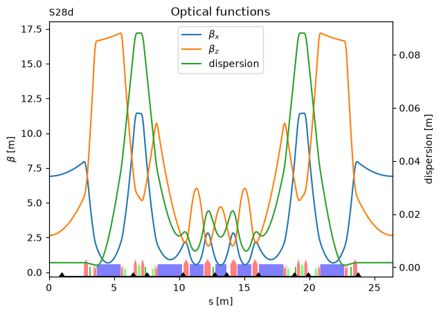
hmba_lattice.plot_beta()

(<Axes: title={'left': 'S28d', 'center': 'Optical functions'}, xlabel='s [m]', ylabel='$\\beta$ [m]'>,
 <Axes: ylabel='dispersion [m]'>,
 <Axes: >)

The first BPM is moved to a location where \(\beta_y=3.0\)

Restore the lattice

dr1.Length = l1
dr2.Length = l2

Method 2: derivating the VariableBase class

We define a new variable class which will act on the two elements and fulfil the constraint

Define a variable coupling two drift lengths so that their sum is constant:

class ElementShifter(VariableBase):
    def __init__(self, dr1, dr2, total_length=None, **kwargs):
        """Varies the length of the elements *dr1* and *dr2*
        keeping the sum of their lengths equal to *total_length*.

        If *total_length* is None, it is set to the initial total length
        """        
        # store indexes of the 2 variable elements
        self.dr1 = dr1
        self.dr2 = dr2
        # store the initial total length
        if total_length is None:
            total_length = dr1.Length + dr2.Length
        self.length = total_length
        super().__init__(bounds=(0.0, total_length), **kwargs)

    def _setfun(self, value, ring=None):
        dr1.Length = value
        dr2.Length = self.length - value

    def _getfun(self, ring=None):
        return  dr1.Length

This method is more powerful, for instance by allowing processing in the init method.

Create a variable moving the monitor BPM_01

var0 = ElementShifter(dr1, dr2, name='DR_01', total_length=ltot)

Run the matching

variables = VariableList([var0])
constraints = ObservableList([obs1], ring=hmba_lattice)
match(hmba_lattice, variables, constraints, verbose=1)

1 constraints, 1 variables, using method trf

`gtol` termination condition is satisfied.
Function evaluations 8, initial cost 2.6515e+00, final cost 9.6605e-27, first-order optimality 9.88e-14.

Constraints:

    location              Initial            Actual         Low bound        High bound         deviation 
beta[y]
    BPM_01                5.30283               3.0               3.0               3.0        1.0924e-08 

Variables:

        Name      Initial          Final        Variation

       DR_01    2.651400e+00    9.693778e-01   -1.682022e+00

Show the modified lattice

for elem in hmba_lattice.select([2,3,4]):
    print(elem)

Drift:
       FamName: DR_01
        Length: 0.969377825260562
    PassMethod: DriftPass
Monitor:
       FamName: BPM_01
        Length: 0.0
    PassMethod: IdentityPass
        Offset: [0 0]
       Reading: [0 0]
      Rotation: [0 0]
         Scale: [1 1]
Drift:
       FamName: DR_02
        Length: 1.7245741747394379
    PassMethod: DriftPass

hmba_lattice.plot_beta()

(<Axes: title={'left': 'S28d', 'center': 'Optical functions'}, xlabel='s [m]', ylabel='$\\beta$ [m]'>,
 <Axes: ylabel='dispersion [m]'>,
 <Axes: >)