Response matrices

import at
import numpy as np
import math
from pathlib import Path
from importlib.resources import files, as_file
from timeit import timeit
from at.future import VariableList, RefptsVariable

with as_file(files("machine_data") / "hmba.mat") as path:
    hmba_lattice = at.load_lattice(path)

for sx in hmba_lattice.select(at.Sextupole):
    sx.KickAngle=[0,0]
hmba_lattice.enable_6d()

ring = hmba_lattice.repeat(8)

A ResponseMatrix object defines a general-purpose response matrix, based on a VariableList of attributes which will be independently varied, and an ObservableList of attributes which will be recorded for each variable step.

ResponseMatrix objects can be combined with the “+” operator to define combined responses. This concatenates the variables and the observables.

The module also defines two commonly used response matrices: OrbitResponseMatrix for circular machines and TrajectoryResponseMatrix for beam lines. Other matrices can be easily defined by providing the desired Observables and Variables to the ResponseMatrix base class.

General purpose response matrix

Let’s take the horizontal displacements of all quadrupoles as variables:

variables = VariableList(RefptsVariable(ik, "dx", name=f"dx_{ik}", delta=.0001)
                        for ik in ring.get_uint32_index(at.Quadrupole))

Variable names are set to dx_nnnn where nnnn is the index of the quadrupole in the ring.

Let’s take the horizontal positions at all beam position monitors as observables:

observables = at.ObservableList([at.OrbitObservable(at.Monitor, axis='x')])

We have a single Observable named orbit[x] by default, with multiple values.

Instantiation

resp_dx = at.ResponseMatrix(ring, variables, observables)

At that point, the response matrix is empty.

Matrix Building

A general purpose response matrix may be filled by several methods:

1. Direct assignment of an array to the response property. The shape of the array is checked,

2. load() loads data from a file containing previously saved values or experimentally measured values,

3. build_tracking() computes the matrix using tracking,

4. For some specialized response matrices build_analytical() is available.

resp_dx.build_tracking(use_mp=True)

array([[ 16.94897864,  -7.67022307,   2.50968594, ...,   5.3125638 ,
         -5.57239476,  14.39501938],
       [-10.6549627 ,   3.59085167,  -6.21666755, ...,  -2.46632948,
          8.42841189, -18.50171186],
       [-10.99744814,   3.91741643,  -5.60080281, ...,  -2.73604877,
          7.61448343, -17.01886021],
       ...,
       [-17.0182359 ,   7.61358522,  -2.73824047, ...,  -5.60018031,
          3.92050176, -11.00305834],
       [-18.50166601,   8.42772786,  -2.46888914, ...,  -6.21619686,
          3.59444354, -10.66160249],
       [ 14.38971545,  -5.56943704,   5.31320321, ...,   2.50757509,
         -7.6711941 ,  16.94982252]], shape=(80, 128))

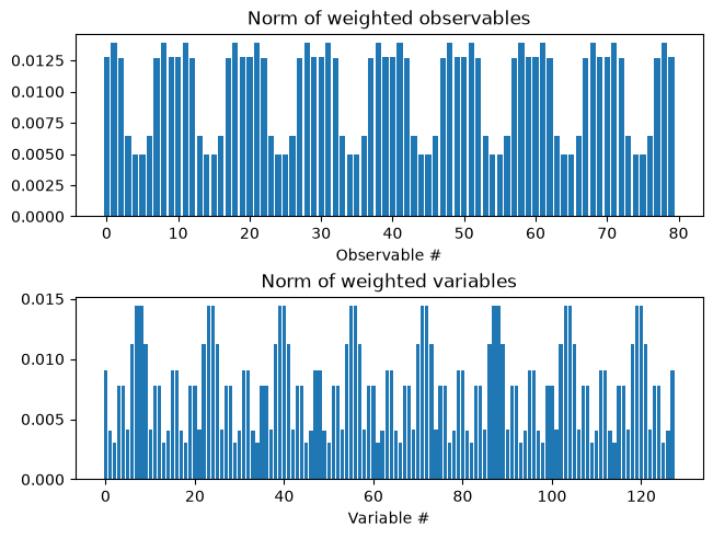
Matrix normalisation

To be correctly inverted, the response matrix must be correctly normalised: the norms of its columns must be of the same order of magnitude, and similarly for the rows.

Normalisation is done by adjusting the weights \(w_v\) for the variables \(\mathbf{V}\) and \(w_o\) for the observables \(\mathbf{O}\). With \(\mathbf{R}\) the response matrix:

\[ \mathbf{O} = \mathbf{R} . \mathbf{V}\]

The weighted response matrix \(\mathbf{R}_w\) is:

\[ \frac{\mathbf{O}}{w_o} = \mathbf{R}_w . \frac{\mathbf{V}}{w_v}\]

The \(\mathbf{R}_w\) is dimensionless and should be normalised. This can be checked using:

• check_norm() which prints the ratio of the maximum / minimum norms for variables and observables. These should be less than 10.

• plot_norm()

Both natural and weighted response matrices can be retrieved with the response() and weighted_response() properties.

resp_dx.plot_norm()

max/min Observables: 2.8352796928879394
max/min Variables: 4.768846272300127

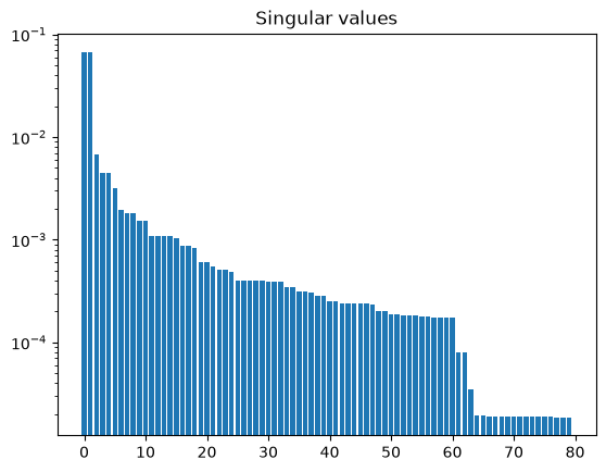
Matrix pseudo-inversion

The solve() method computes the singular values of the weighted response matrix and its pseudo-inverse.

resp_dx.solve()

We can plot the singular values:

resp_dx.plot_singular_values()

After solving, correction is available, for instance with

• correction_matrix() which returns the correction matrix (pseudo-inverse of the response matrix),

• get_correction() which returns a correction vector when given observed values,

• correct() which computes and optionally applies a correction for the provided Lattice.

Exclusion of variables and observables

Variables may be added to a set of excluded values, and similarly for observables. Excluding an item does not change the response matrix. The values are excluded from the pseudo-inversion of the response, possibly reducing the number of singular values. After inversion, the correction matrix is expanded to its original size by inserting zero lines and columns at the location of excluded items. This way:

• error and correction vectors keep the same size independently of excluded values,

• excluded error values are ignored,

• excluded corrections are set to zero.

Exclusion of variables

Excluded variables are selected by their name or their index in the variable list:

resp_dx.exclude_vars(0, "dx_9", "dx_47", -1)

Where -1 refers to the last variable.

Exclusion of observables

Observables are selected by their name or their index in the observable list. In addition, for ElementObservable observables, we need to specify a refpts to identify which item in the array will be excluded.

Let’s exclude all Monitors with name BPM_07:

resp_dx.exclude_obs(obsid="orbit[x]", refpts="BPM_07")

Or by using the observable index:

resp_dx.exclude_obs(obsid=0, refpts="BPM_07")

Or even, since there is a single observable and obsid defaults to 0:

resp_dx.exclude_obs(refpts="BPM_07")

After excluding items, the pseudo-inverse is discarded so one must recompute it again:

resp_dx.solve()
resp_dx.plot_singular_values()

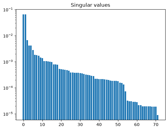
There are now only 72 singular values instead of 80 (number of active monitors).

The excluded items can be retrieved with the excluded_obs and excluded_vars properties:

print(resp_dx.excluded_obs)
print(resp_dx.excluded_vars)

{'orbit[x]': array([ 79, 200, 321, 442, 563, 684, 805, 926], dtype=uint32)}
['dx_5', 'dx_9', 'dx_47', 'dx_964']

The exclusion masks can be reset using reset_vars() and reset_obs().

Orbit response matrix

An OrbitResponseMatrix defines its observables as instances of OrbitObservable and its variables as KickAngle attributes of elements.

Instantiation

By default, the observables are all the Monitor elements, and the variables are all the elements having a KickAngle attribute. This is equivalent to:

resp_v = at.OrbitResponseMatrix(ring, "v", bpmrefs = at.Monitor,
                                steerrefs = at.checkattr("KickAngle"))

The variable elements must have the KickAngle attribute used for correction. It’s available for all magnets, though not present by default except in Corrector magnets. For other magnets, the attribute should be explicitly created.

There are options in OrbitResponseMatrix to include the RF frequency in the variable list, and the sum of correction angles in the list of observables:

resp_h = at.OrbitResponseMatrix(ring, "h", cavrefs=at.RFCavity, steersum=True)
print(resp_h.shape)

(81, 49)

Matrix building

OrbitResponseMatrix has a build_analytical() build method, using formulas from [1].

resp_h.build_analytical()

array([[-8.54870374e+00, -1.81104969e+01, -1.21497454e+01, ...,
        -2.85830326e+01, -1.60772960e+01, -5.75838151e-08],
       [ 1.85290756e+01,  3.16574224e+01,  1.82799745e+01, ...,
         1.90656557e+01,  8.85865108e+00, -2.68128309e-06],
       [ 1.68213604e+01,  2.87634523e+01,  1.65301788e+01, ...,
         1.94726063e+01,  9.44097149e+00, -2.44436213e-06],
       ...,
       [ 8.84897619e+00,  1.90656922e+01,  1.29411619e+01, ...,
         3.16578009e+01,  1.85390265e+01, -2.68138514e-06],
       [-1.60775574e+01, -2.85833742e+01, -1.65903209e+01, ...,
        -1.81113028e+01, -8.54900471e+00, -5.76356368e-08],
       [ 1.00000000e+00,  1.00000000e+00,  1.00000000e+00, ...,
         1.00000000e+00,  1.00000000e+00,  0.00000000e+00]],
      shape=(81, 49))

Matrix normalisation

This is critical when including the RF frequency response which is not commensurate with steerer responses. Similarly for rows, the sum of steerers is not commensurate with monitor readings.

By default, the normalisation is done automatically by adjusting the RF frequency step and the weight of the steerer sum based on an approximate analytical response matrix. Explicitly specifying the cavdelta and stsumweight prevents this automatic normalisation.

After building the response matrix, and before solving, normalisation may be applied with the normalise() method. The default normalisation gives a higher priority to RF response and steerer sum.

Trajectory response matrix

A TrajectoryResponseMatrix defines its observables as instances of TrajectoryObservable and its variables as KickAngle attributes of elements.

Instantiation

By default, the observables are all the Monitor elements, and the variables are all the elements having a KickAngle attribute. This is equivalent to:

resp_v = at.TrajectoryResponseMatrix(lattice, "v", bpmrefs = at.Monitor,
                                     steerrefs = at.checkattr("KickAngle"))

The variable elements must have the KickAngle attribute used for correction. It’s available for all magnets, though not present by default except in Corrector magnets. For other magnets, the attribute should be explicitly created.

resp_h = at.TrajectoryResponseMatrix(ring, "h")
print(resp_h.shape)

(80, 48)

References

---

[1]

A. Franchi, S.M. Liuzzo, Z. Marti, “Analytic formulas for the rapid evaluation of the orbit response matrix and chromatic functions from lattice parameters in circular accelerators”, arXiv:1711.06589 [physics.acc-ph]