at.plot.observables#
Functions
|
Plot element observables along a lattice. |
- plot_observables(ring, obsleft, *obsright, s_range=None, axes=None, xlabel='', ylabel='', title='', slices=400, dipole={}, quadrupole={}, sextupole={}, multipole={}, monitor={}, labels=None, **kwargs)[source]#
Plot element observables along a lattice.
- Parameters:
ring (Lattice) – Lattice description
obsleft (ObservableList) – List of
ElementObservableplotted against the left axis. if refpts isAll, a line is drawn. Otherwise, markers are drawn. It is recommended to use Observables with scalar values. Otherwise, all the values are plotted but share the same line properties and legend,obsright (ObservableList) – Optional list of
ElementObservableplotted against the right axis,axes (Axes | None) –
Axesin which the observables are plotted. ifNone, a new figure is created,s_range (tuple[float, float] | None) – Lattice range of interest, default: whole lattice,
slices (int) – Number of lattice slices for getting smooth curves. Default: 400.
xlabel (str) – x-axis label. Default:
s [m].ylabel (str) – y-axis label. Default:
ObservableList.axis_label.title (str) – Plot title,
The following keywords are transmitted to the
plot_synopt()function.They apply to the main (left) axis and are ignored when plotting in exising axes:- Keyword Arguments:
labels (Refpts) – Select elements for which the name is displayed. Default:
None,dipole (dict) – Dictionary of properties overloading the default properties of the dipole representation. Example:
{"facecolor": "xkcd:electric blue"}. IfNone, dipoles are not shown.quadrupole (dict) – Same definition as for dipole,
sextupole (dict) – Same definition as for dipole,
multipole (dict) – Same definition as for dipole,
monitor (dict) – Same definition as for dipole.
- Returns:
axes – tuple of
Axes. Contains 2 elements if there is a plot on the right y-axis, 1 element otherwise.
Note
The legend of the plot is controlled by the
Observable.labelattributes. Default values are provided, but labels may explicitly set.Labels may contain LaTeX math code. Example:
"$\beta_x$"will appear as “\(\beta_x\)”.Labels starting with an underscore do not appear in the legend.
Examples
Minimal example using default values:
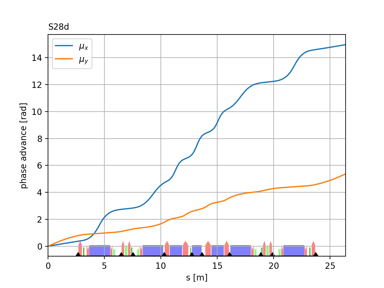
>>> obsmu = at.ObservableList(
...     [
...         at.LocalOpticsObservable(at.All, "mu", plane=0),
...         at.LocalOpticsObservable(at.All, "mu", plane=1),
...     ]
... )
>>>
>>> (ax1,) = at.plot_observables(ring, obsmu)
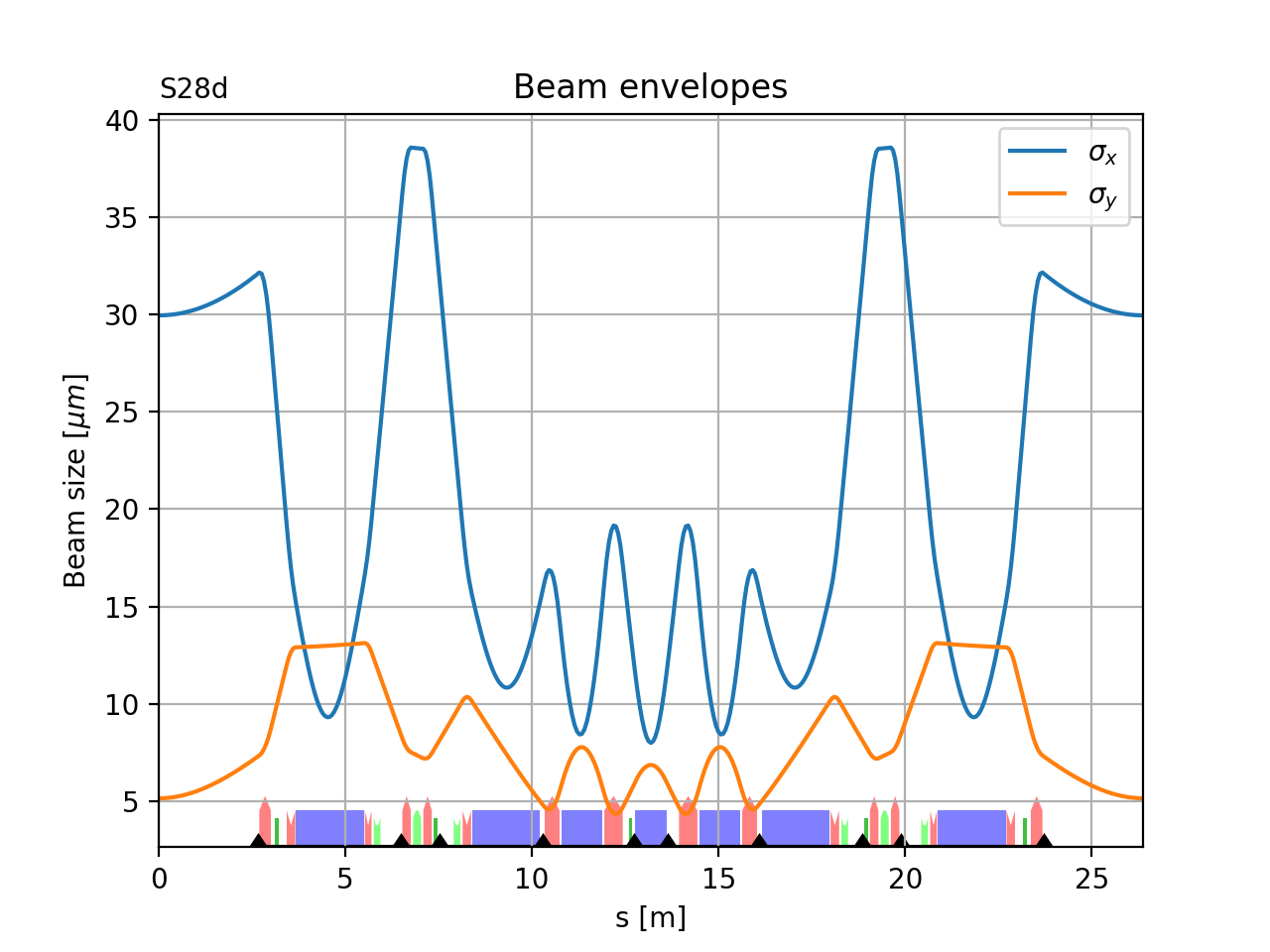
This example demonstrates the use of the postfun post-processing attribute of observables to plot the beam envelopes for arbitrary emitttance values:
>>> # Define the emittances
>>> emit_x = 130.0e-12
>>> emit_y = 10.0e-12
>>>
>>> # beam size computation
>>> sigma_x = lambda x: 1.0e6 * np.sqrt(x * emit_x)  # result in um
>>> sigma_y = lambda y: 1.0e6 * np.sqrt(y * emit_y)  # result in um
>>>
>>> # Observables
>>> obsenv = at.ObservableList(
...     [
...         at.LocalOpticsObservable(
...             at.All, "beta", plane="x", postfun=sigma_x, label=r"$\sigma_x$"
...         ),
...         at.LocalOpticsObservable(
...             at.All, "beta", plane="y", postfun=sigma_y, label=r"$\sigma_y$"
...         ),
...     ]
... )
>>> (ax2,) = at.plot_observables(
...     ring, obsenv, ylabel=r"Beam size [${\mu}m$]", title="Beam envelopes"
... )
>>> )