at.plot.response#

Plot Observable values as a function of a Variable.

Functions

plot_response(var, rng, obsleft, *obsright)

Plot Observable values as a function of a Variable.

plot_response(var, rng, obsleft, *obsright, axes=None, xlabel='', ylabel='', **kwargs)[source]#

Plot Observable values as a function of a Variable.

Parameters:

var (VariableBase) – Variable object,
rng (Iterable[float]) – range of variation for the variable,
obsleft (ObservableList) – List of Observables plotted on the left axis. It is recommended to use Observables with scalar values. Otherwise, all the values are plotted but share the same line properties and legend,
obsright (ObservableList) – Optional list of Observables plotted on the right axis.
axes (Axes | None) – Axes object in which the figure is plotted. If None, a new figure is created.
xlabel (str) – x-axis label. Default: variable name.
ylabel (str) – y-axis label. Default: ObservableList.axis_label.

Additional keyword arguments are transmitted to the Axes creation function.They apply to the main (left) axis and are ignored when plotting in exising axes:

Keyword Arguments:

title (str) – Plot title,
ylim (tuple) – Y-axis limits,
* – for other keywords see add_subplot

Returns:

axes – tuple of Axes. Contains 2 elements if there is a plot on the right y-axis, 1 element otherwise.

Note

The legend of the plot is controlled by the Observable.label attributes. Default values are provided, but labels may explicitly set.

Labels may contain LaTeX math code. Example: "$\beta_x$" will appear as “$\beta_x$”.

Labels starting with an underscore do not appear in the legend.

Example

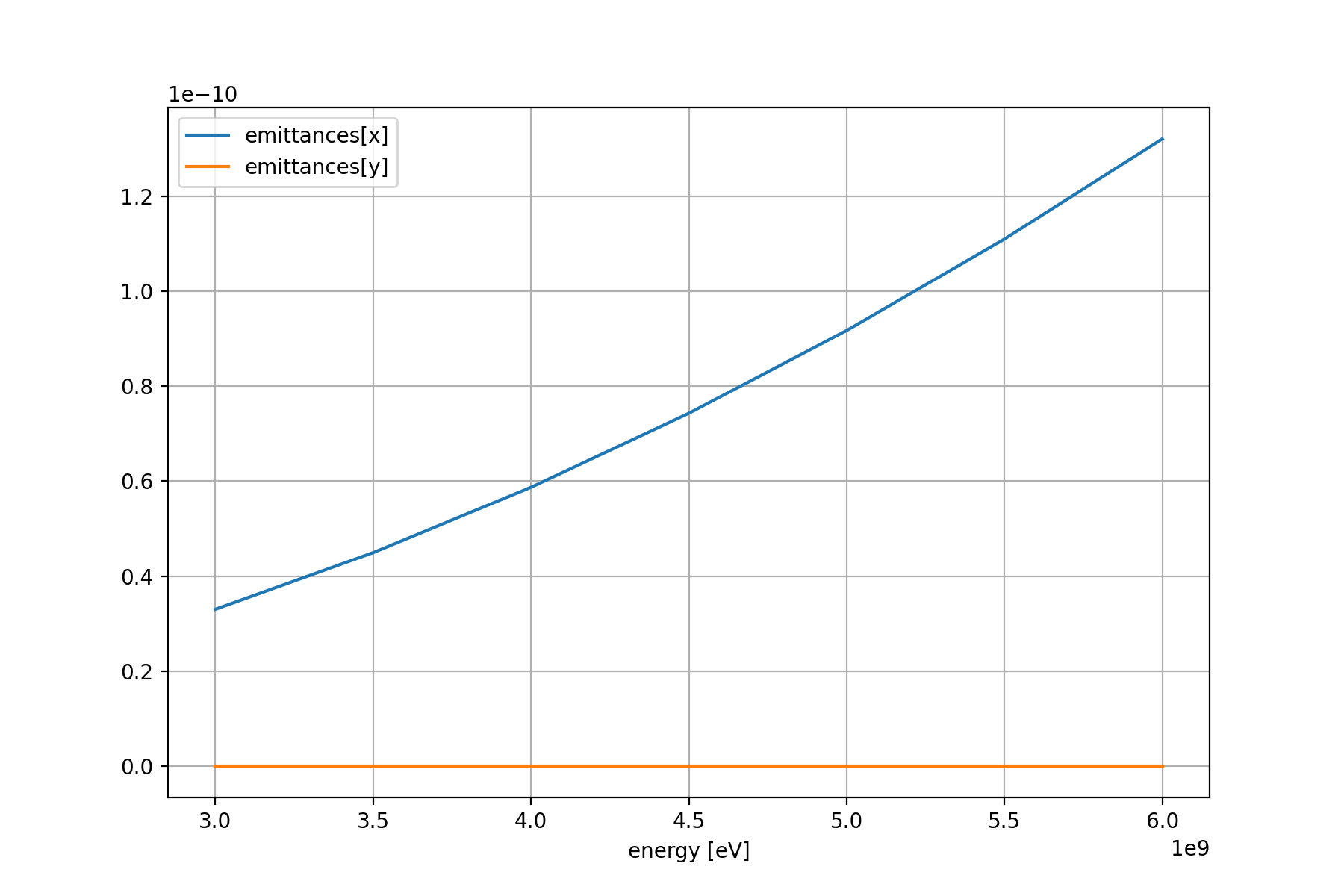
Minimal example using only default values:

>>> obsl = at.ObservableList(
...     [at.EmittanceObservable("emittances", plane="x")],
...     ring=ring,
... )
>>> obsr = at.ObservableList(
...     [at.EmittanceObservable("sigma_e")],
...     ring=ring,
... )
>>> var = at.AttributeVariable(ring, "energy", name="energy [eV]")
>>> ax1, ax2 = at.plot_response(
...     var, np.arange(3.0e9, 6.01e9, 0.5e9), obsl, obsr
... )
>>>

Example showing the formatting possibilities by:

using the Observable.plot_fmt attribute for line formatting,
using dual y-axis,
using the ylim and title parameters.

>>> obsleft = at.ObservableList(
...     [
...         at.LocalOpticsObservable(
...             [0], "beta", plane="x",
...             plot_fmt={"linewidth": 3.0, "marker": "o"}
...         ),
...         at.LocalOpticsObservable([0], "beta", plane="y", plot_fmt="--"),
...     ],
...     ring=ring,
... )
>>>
>>> obsright = at.ObservableList(
...     [
...         at.GlobalOpticsObservable("tune", plane="x"),
...         at.GlobalOpticsObservable("tune", plane="y"),
...     ],
...     ring=ring,
... )
>>>
>>> var = RefptsVariable(
...     "QF1[AE]", "Kn1L", name="QF1 integrated strength", ring=ring
... )
>>> ax = at.plot_response(
...     var,
...     np.arange(0.732, 0.852, 0.01),
...     obsleft,
...     obsright,
...     ylim=[0.0, 10.0],
...     title="Example of plot_response",
... )

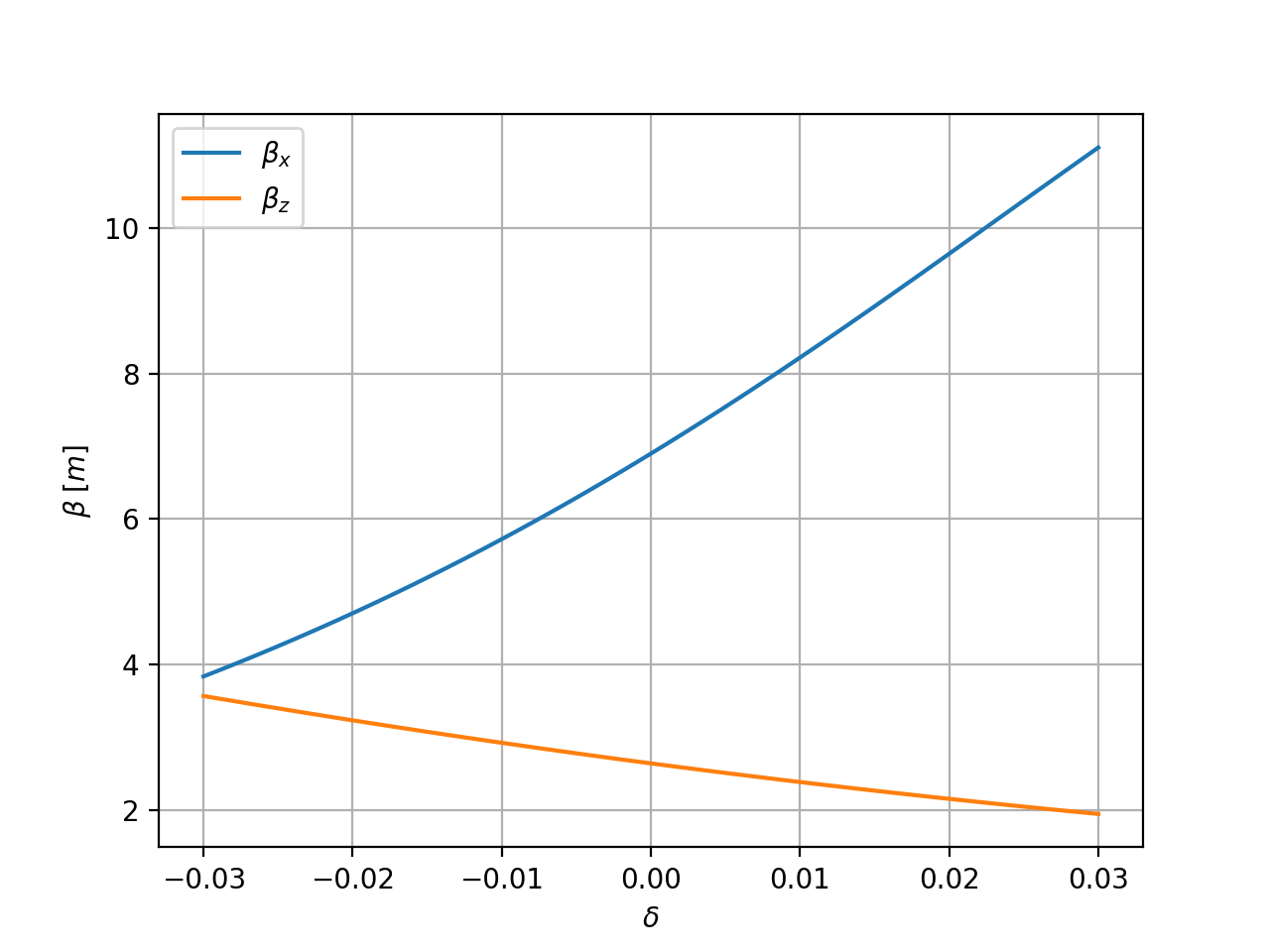
Example varying an evaluation parameter:

>>> obs = at.ObservableList(
...     [
...         at.LocalOpticsObservable([0], "beta", plane="x"),
...         at.LocalOpticsObservable([0], "beta", plane="y"),
...     ],
...     ring=ring,
...     dp=0.0,
... )
>>> var = at.EvaluationVariable(obsleft, "dp", name=r"$\delta$")
>>> ax = at.plot_response(var, np.arange(-0.03, 0.0301, 0.001), obsleft)